Sunday 25 February 2018

ALG 4

This set of ALG 4 tasks might require a somewhat greater understanding of algebra than the previous three ALG tasks, if students are to grasp some of the algebraic relations, especially in their more general form. However, even relative novices should be able to engage with the tasks and construe patterns even if this might be at a more empirical level.
MONDAY: This is the root ALG 4 task for this week. It can be approached in quite an exploratory way - later variants become more focused.
Here it is worth dwelling for a while on the form of the three equations, before sketching any lines. Students who know about the form of linear functions may notice that the greater the slope of the corresponding lines, the higher the point of intersection with the y-axis (ie as m increases, so does c, in y = mx + c). In turn this might suggest that the lines are 'hinged' about a common point, which turns out to be the case.
Students without this kind of knowledge can still engage meaningfully with the task, by sketching the lines given by the equations and examining the result.
-
TUESDAY: In this variant we show the three lines and ask students to explain the fact that they go through a common point, using both algebraic and geometric arguments.
 As can be seen, the lines all go through the point (-3, 0). We can verify this by letting y = 0 in each of the equations and then solving for x, or by solving for x in the general equation y = ax + 3a or y = a(x + 3) after letting y = 0.
We can also explain this in terms of the slope of the lines and the triangle formed by the points with coordinates (-3, 0), (0, 0) and (0, c). We can think of the slope as being the change in y resulting from a change of +1 in the value of x (below). This means if we increase x by +3, in moving from (-3, 0) to the origin, we increase y by +3×m, and hence cut the y axis at (0, 3m).
-
WEDNESDAY: Here we find the common point for the lines given by another family of equations. But this time, rather than listing individual equations, the family is expressed in a general form. This might help students express the previous family in a similar form if they have not already done so (ie, as y = ax + 3a, as mentioned above). Also, as the two forms are very similar, it might help students see how, and perhaps why, the general form relates to the lines' common point.
[It might be argued that the form y = a(x – 2) is more salient than the given form y = ax – 2a, even though it diverges from the familiar y = mx + c form, as it immediately becomes apparent that x = 2 when y = 0, regardless of the value of a.]
-
THURSDAY: Here we consider another family of equations whose general form, at least at first sight, seems rather different from the form of the two families we've considered so far. It turns out that the common point is not on the x-axis this time.
There are several ways of writing the general form of the family of equations, for example these:
y = ax + (3 – a), y = a(x – 1) + 3, y – 3 = a(x – 1).
What are the affordances of each?
-
FRIDAY: Here we reverse the process, by asking for the family of lines that goes through a specific point.
 We can approach this in different ways. One way is to find the equations of some specific lines through (2, 5) and look for a pattern. Another would be to look back at Thursday's task and see what's general about it, ie how does the general equation (in whatever form) relate to the common point?
Another way of thinking about this is to consider lines through the origin (ie of the form y = ax) and to think of translating the lines 2 across and 3 up - how do these steps transform the equation?
An obvious extension of the task would be to consider a general point, with coordinates (u, v), say. If you've managed to solve the task for (2, 5), this should be fairly easy ....

Sunday 18 February 2018

ALG 3

In this week's set of tasks we try to get a better feel for a linear function by comparing it with a non-linear function. We see that as the independent variable changes at a steady rate, the values of the functions change at different rates, with one of them changing steadily.
The functions are set in a geometric context and we compare them geometrically (in two different ways, one of which is much more salient than the other), by expressing them symbolically, and by looking at numerical values in an ordered table.
-
MONDAY: This is the root task for the week. It can be quite tricky ....
After students have drawn the shape for u = 3, you might want to show this:
-
TUESDAY: Here we compare the area of our cross-shape with the area of another cross-shape:
You might want to present this on two separate slides, starting with the edited version below, so that students are not channeled too soon into answering the more structured second part. It is worth giving students plenty of time to explore the question, "Which shape has the larger area?".
After students have explored the task, they can check their hunches and confirm their insights with this Dynamic crosses movie. Some clips from the movie are shown below:
-
WEDNESDAY: Here we repeat Tuesday’s task but we treat the cross-shapes as the nets of two open boxes. 
For one of the boxes, as u increases, the height of the box increases but the (square) base stays the same; for the other box, its base gets larger (in both dimensions) but the height stays the same. Thus one box changes in two dimensions simultaneously, while the other changes in only one. 
These changes are far less obvious when one just looks at the 2D nets, unless one re-configures them. For example, the first cross-shape is changing in two directions as u changes. However, if one cuts and re-joins the net like this (below), the change can be seen to occur in just one dimension.
We can do the same for the net of the other box. As u increases, the net expands in two dimensions, because of the u by u square (tinted).
-
THURSDAY:This is Thursday's variant on the ALG 3 task. By now, students will, hopefully, have developed a good feel for how the areas of the two cross-shapes change with u: eg, that the first shape's area increases steadily for steady increases in u; and that the second shape's area changes more and more rapidly as u increases, and so, though its area is smaller for values like u = 2, it overtakes the other area at some point, namely when u gets past 5.
So in today's task, we represent the areas symbolically, with the aim of making these ideas about the changing areas more explicit and, conversely, giving meaning to the resulting algebraic expressions. This may also help students to get a better sense of the general form of what turn out to be linear and quadratic expressions.
-
FRIDAY: Here we try to consolidate some of the burgeoning ideas by revisiting the numerical values found in Tuesday's task, and judiciously extending these with the aid of an ordered table.
 A possible next step would be to graph these sets of values - both as a way of illuminating the nature of the (linear and quadratic) relations, and as a way of giving meaning to graphs. And it would be worth relating this to the Dynamic crosses movie (with the mouse over the play/pause button).
The completed table looks like this:
 As we can see, as u increases by 1, 20u+25 increases by the same amount, whether we start from u=5 or u=10, whereas 20u+u2 increases by an increasing amount ....
We can illustrate this with a graph, such as this off-the-peg version from Excel.
The graph raises some interesting questions:
  • The blue line appears to be straight. Is this really the case and what would this mean (algebraically, and in the context of the cross-shape's area)? 
  • The red line seems to consist of ever-steeper line segments. Does this make sense? What if I had chosen different data-points - would I get different line-segments?? 
  • What happens to the two graphs for negative values of u (algebraically, and in terms of the cross-shapes and their areas)?
It can also be illuminating to see how equivalent forms of the algebraic expressions relate to (and can be derived from) the shapes of the crosses. This is for the first cross-shape:
 And this is for the second cross-shape: 


Thursday 15 February 2018

ALG 2

Here is an open version of our ALG 2 root task - a slightly more structured version will appear on Monday, with other variants later in the week.
The task starts with the idea that an unknown can vary, rather than the more common idea in school mathematics that it has a specific value that we want to find.
Also, rather than immediately asking students to perform various actions on the unknown (such as collecting like terms, manipulating or evaluating expressions, forming and solving equations), the task may help students realise that they can sometimes make sense of expressions from the outset - especially in this case, where the given expressions (x and 2x) are fairly simple, and thus might fairly readily lead to an interpretation like 'one angle in the triangle is twice the size of another angle'.
A movie of the triangle can be found here.
-
MONDAY: Here is this week's root task. It is more structured than the version above but it should still help students discern the general relationship between two of the triangle's angles (ie between the expressions x and 2x). Part b) provides a shift towards the use of algebraic procedures, by asking students to find a particular (critical) value of x. We can solve this algebraically by forming the equation x + 2x = 180. However, it is important to acknowledge that we can also find x quite easily by other means, eg trial and improvement.
 We have made two movies showing the triangle as x varies. In one movie the value of x goes up to the 'permissible' value. In the other movie the value of x goes beyond this value: what happens to the triangle when this occurs, and should such values be 'allowed'?!
-
TUESDAY: Like Monday's part b), we don't need formal algebra to solve this variant of ALG 2, but it gives us the opportunity to construct two more equations in x, so it becomes interesting to compare them and to discuss ways in which they can be solved.
 It is also worth engaging with the geometry of the situation. For example, why is the triangle always weighted to the right in the given diagrams? Also, we can see from the given triangles that the value of x will be close to 35 for one of the isosceles triangles, and somewhat less than 50 for the other - do our algebraic approaches confirm this?
-
WEDNESDAY: Having looked for isosceles triangles, this variant involves finding values of x for which the triangle is right-angled:
We can find x by using trial and improvement, say, but we can also proceed algebraically by forming equations to represent the geometric relations resulting from angle B or angle C being a right angle. This gives 2x = 90 and x + 2x = 90 (or x + 2x + 90 = 180). Similarly, we can form equations for the earlier variants: x + 2x = 180 (ALG 2A), x + 2x + 2x = 180 and x + x + 2x = 180 (ALG 2B). These equations are all fairly easy to solve, but what is particularly nice about the more complex ones is that we may be able to persuade students of their utility: by forming and writing down equations we can ease the strain on our working memory.
It can also be useful to discuss and compare different ways of solving the equations, eg by inspection, by trial and improvement, or by transforming the equations.
-
THURSDAY: Here we change the relationship between the base angles of the triangle from x˚, 2x˚ to x˚, 4x˚. This gives students a chance to recap on earlier ideas and methods, as well as perhaps starting to think about how changes in the angle relationship might affect the size of the various angles that we are trying to find.
Thursday enjoyed a couple of bonus tasks (below). The first can be varied in quite nice ways. The other [based on a seminal idea from David Fielker, writing some years ago in Mathematics Teaching] says something about the freedom that symbolic algebra can give us.
And here's another bonus (actually posted on Friday) which continues the regular polygon theme:
-
FRIDAY: This is our final (for now?) ALG 2 variant. It gives plenty of scope for consolidation and for exploring the relationship between the base angles, which is expressed here in a more general way (with the aid of parameters a and b). Let us know what you or your students find.

-
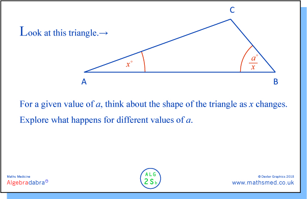
SUNDAY Supplement: Here's a set of three tasks still involving the base angles of a triangle but where there's an inverse proportional relationship. Some of the resulting triangle-families can be quite surprising.
Here's the first task (below). Part a) is to get students to start thinking about the scenario. The given information means that a/20 = 50, so a = 1000. It might seem surprising that a relation involving '1000' works in the context of triangles, where the interior angle sum is a mere 180˚. Of course, the relation ∠A = x˚, ∠B = 1000˚/x doesn't work for all values of x. For example, if x = 1, then ∠B would be 1000˚. However it turns out the relation works for this range of values (approximately): 
6 ≤ x ≤ 174.
It is worth spending quite a lot of time on part b)i, to get a feel for how the base angles, and the overall shape of the triangle, change. The triangle turns out to be fairly 'flat'. When x is 'small', a change in x produces a rapid change in ∠B; when x is fairly 'large' ∠B seems to change hardly at all. A movie of the changing triangle can be found here.
A good way to start part b)ii is to adopt a visual approach, eg by running the aforementioned movie and pausing it when the triangle looks to be isosceles. This happens in three places. A more precise estimate can then be found by using a numerical approach, which can be made more and more precise with the aid of a spreadsheet (with a column for x, for 1000/x and for 180 – x – 1000/x).
In the isosceles case where ∠A = ∠B, x = √1000. The value of x for the other two cases (∠A = ∠C and ∠C = ∠B) can be found algebraically by forming an equation in x and writing it in the usual quadratic form. However, it doesn't factorise....
-
Here's the second Sunday Supplement task. This is very exploratory. You might want to start by seeing what happens with some fairly 'random' values of a, and then try some more 'informed' values.
After some explorations, you might want to look at two further movies, where a = 100 and a = 1.
The choice of '100' is very deliberate and you might like to predict what effect this has on the shape of the triangle. The effect of choosing a = 1 is very strange.... - but the movie won't win any Oscars.
-
The third Sunday Supplement:
In this task the numbers are nicer. You might be able to see the value of x for which ∠A = ∠B. The value of x for the other two isosceles cases (∠A = ∠C and ∠C = ∠B) can be found by forming a quadratic equation which this time does factorise. Or you could adopt a visual/numeric approach again, perhaps with the aide of this movie, or this second version which provides a trace of vertex C.

Sunday 11 February 2018

Singalong

All together now ....
-
[with thanks to Steve Miller and The Steve Miller Band]
[and to Wren]
-

Sunday 4 February 2018

ALG 1


MONDAY: This is the ‘root’ task for the week.
The task is designed to help students focus on the structure of the equation, rather than to reach for a familiar procedure for solving it (be it an informal strategy like trial and improvement or the use of formal transformation rules). We are not really interested in the solution per se - although it is fairly easy to find, if one uses the given information and observes the equation's structure.
-
TUESDAY: Tweaking a term in an equation can help us see what role the term plays in the equation and how it interacts with other terms. Here's another tweak of the original equation, one whose effect is relatively easy to see:
You or students might like to think of some other tweaks - which ones seem easy to construe, and which are more opaque?
-
WEDNESDAY: The tweak lined up for the middle of the week is nice and simple. Actually, I've decided on an extra tweak. Both still quite simple, but they seem to work in subtly different ways. What's going on?!
It might strike us as odd (at least momentarily), that doing the same thing additively to the terms 77 and 203 has no effect, while multiplicatively it does ....
-
THURSDAY: This is Thursday's variant. If it seems too simple, you could change 42 to 84, say, or wouldn't that make enough difference? I'd be interested to know.
-
FRIDAY: Here's the last ALG 1 variant (for now?). With some classes, you might decide to start with an open task such as this, rather than the earlier, more closed variants.
And you might (at some stage) want something more open still, eg along the lines of "Change one of the numbers in the equation - what does this do to the solution?". You might also want to investigate equations with a different form from ax + b = c.

Thursday 1 February 2018

About this site


This blog was started on 1 February 2018. Its aim was to publish tasks designed to help school students get a better feel for algebra.
The plan was to post a new task at the beginning of a week, and then to post variations of the task during the week, together with comments and guidance. I managed to carry this through for 20 weeks, resulting in 20 lots of 5 related tasks, ie 100 tasks in all.

About a year later (June 2019), an edited version of the blog was published in the UK as an A5, spiral-bound, 129-page book by the Association of Teachers of Mathematics (ATM). It can be purchased from ATM and costs £12 for members of ATM, £16 for non-members. The book comes with a high-definition pdf file of SLIDES showing all the tasks (and other images) from the book, along with a link for downloading a set of 17 QuickTime movies that support some of the tasks.

You can read more about the book HERE.